Convergence In Probability Using Python

I’m going over Chapter 5 in Casella and Berger’s (CB) “Statistical Inference”, specifically Section 5.5: Convergence Concepts, and wanted to document the topic of convergence in probability with some plots demonstrating the concept.

From CB, we have the definition of convergence in probability: a sequence of random variables $X_{1}, X_{2}, ... X_{n}$ converges in probability to a random variable $X$ , if for every $\epsilon > 0$ ,

$\begin{align} \lim_{n \to \infty} P(| X_{n} - X | \geq \epsilon) = 0 \\ \end{align}$

Intuitively, this means that, if we have some random variable $X_{k}$ and another random variable $X$ , the absolute difference between $X_{k}$ and $X$ gets smaller and smaller as $k$ increases. The probability that this difference exceeds some value, $\epsilon$ , shrinks to zero as $k$ tends towards infinity. Using convergence in probability, we can derive the Weak Law of Large Numbers (WLLN):

$\begin{align} \lim_{n \to \infty} P(|\bar{X}_{n} - \mu | \geq \epsilon) = 0 \end{align}$

which we can take to mean that the sample mean converges in probability to the population mean as the sample size goes to infinity. If we have finite variance (that is $Var(X) < \infty$ ), we can prove this using Chebyshev’s Law

$\begin{align} &= P(|\bar{X}_{n} - \mu | \geq \epsilon) \\ &= P((\bar{X}_{n} - \mu)^{2} \geq \epsilon^{2}) \leq \frac{E\Big[(\bar{X}_{n} - \mu)^{2}\Big]}{\epsilon^{2}} \\ &= P((\bar{X}_{n} - \mu)^{2} \geq \epsilon^{2}) \leq \frac{Var(\bar{X_{n}})}{\epsilon^{2}} \\ &= P((\bar{X}_{n} - \mu)^{2} \geq \epsilon^{2}) \leq \frac{\sigma^{2}}{n^{2}\epsilon^{2}} \end{align}$

where $\frac{\sigma^{2}}{n^{2} \epsilon^{2}} \rightarrow 0$ as $n \rightarrow \infty$ . Intuitively, this means, that the sample mean converges to the population mean – and the probability that their difference is larger than some value is bounded by the variance of the estimator. Because we showed that the variance of the estimator (right hand side) shrinks to zero, we can show that the difference between the sample mean and population mean converges to zero.

We can also show a similar WLLN result for the sample variance using Chebyshev’s Inequality, as:

$\begin{align} S_{n}^{2} = \frac{1}{n-1} \sum_{i=1}^{n} (X_{i} - \bar{X}_{n})^{2} \end{align}$

using the unbiased estimator, $S_{n}^{2}$ , of $\sigma^{2}$ as follows:

$\begin{align} P(|S_{n}^{2} - \sigma^{2}| \geq \epsilon) \leq \frac{E\Big[(S_{n}^{2} - \sigma^{2})^{2}\Big]}{\epsilon^{2}} = \frac{Var(S_{n}^{2})}{\epsilon^{2}} \end{align}$

so all we need to do is show that $Var(S_{n}^{2}) \rightarrow 0$ as $n \rightarrow \infty$ .

Let’s have a look at some (simple) real-world examples. We’ll start by sampling from a $N(0,1)$ distribution, and compute the sample mean and variance using their unbiased estimators.

# Import numpy and scipy libraries
import numpy as np
from scipy.stats import norm

%matplotlib inline
import matplotlib.pyplot as plt

plt.rc('text', usetex=True)

# Generate set of samples sizes
samples = np.concatenate([np.arange(0, 105, 5), 
                          10*np.arange(10, 110, 10),
                         100*np.arange(10, 210, 10)])

# number of repeated samplings for each sample size
iterations = 500

# store sample mean and variance
means = np.zeros((iterations, len(samples)))
vsrs = np.zeros((iterations, len(samples)))

for i in np.arange(iterations):
    for j, s in enumerate(samples):
        
        # generate samples from N(0,1) distribution
        N = norm.rvs(loc=0, scale=1, size=s)
        mu = np.mean(N)
        
        # unbiased estimate of variance
        vr = ((N - mu)**2).sum()/(s-1)

        means[i, j] = mu
        vsrs[i, j] = vr

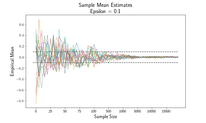
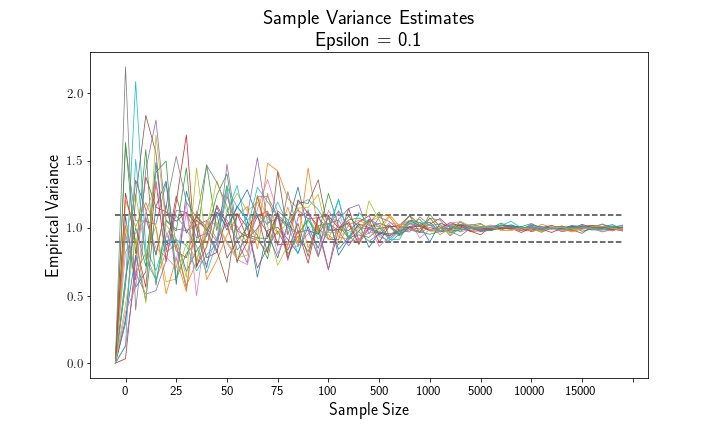
Let’s have a look at the sample means and variances as a function of the sample size. Empirically, we see that both the sample mean and variance estimates converge to their population parameters, 0 and 1.

Sample mean estimates as a function of sample size.

Sample variance estimates as a function of sample size.

Below is a simple method to compute the empirical probability that an estimate exceeds the epsilon threshold.

def ecdf(data, pparam, epsilon):
    
    """
    Compute empirical probability P( |estimate - pop-param| < epsilon).
    
    Parameters:
    - - - - -
    data: array, float
        array of samples
    pparam: float
        true population parameter
    epsilon: float
        threshold value
    """
    
    compare = (np.abs(data - pparam) < epsilon)
    prob = compare.mean(0)
    
    return prob

# test multiple epsilon thresholds
e = [0.9, 0.75, 0.5, 0.25, 0.1, 0.05, 0.01]

mean_probs = []
vrs_probs = []
# compute empirical probabilities at each threshold
for E in e:
    mean_probs.append(1 - ecdf(means, pparam=0, epsilon=E))
    vrs_probs.append(1-ecdf(vsrs, pparam=1, epsilon=E))

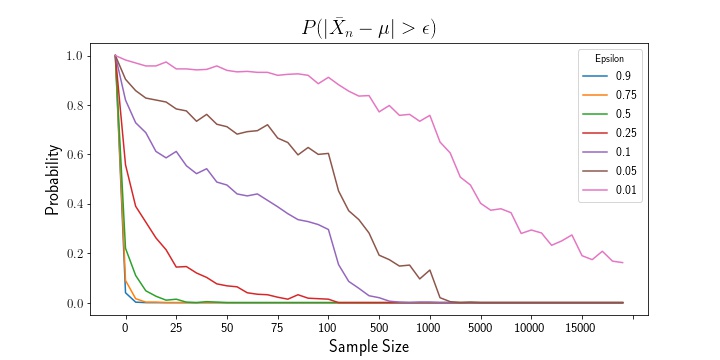
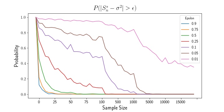
Empirical probability that mean estimate exceeds population mean by epsilon.

Empirical probability that variance estimate exceeds population variance by epsilon.

The above plots show that, as sample size increases, the mean estimator and variance estimator both converge to their true population parameters. Likewise, examining the empirical probability plots, we can see that the probability that either estimate exceeds the epsilon thresholds shrinks to zero as the sample size increases.

If we wish to consider a stronger degree of convergence, we can consider convergence almost surely, which says the following:

$\begin{align} P(\lim_{n \to \infty} |X_{n} - X| \geq \epsilon) = 0 \\ \end{align}$

which considers the entire joint distribution of estimates $( X_{1}, X_{2}...X_{n}, X)$ , rather than all pairwise estimates $(X_{1},X), (X_{2},X)... (X_{n},X)$ – the entire set of estimates must converge to $X$ as the sample size approaches infinity.

← Previous Post Next Post →