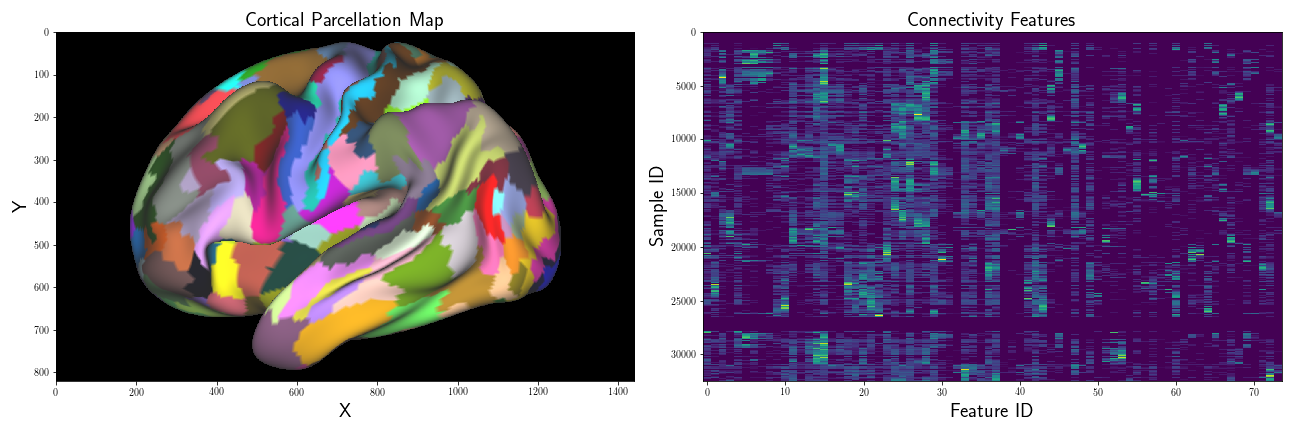
Mahalanobis Distance: A Distributional Exploration of Brain Connectivity

For one of the projects I’m working on, I have an array of multivariate data relating to brain connectivity patterns. Briefly, each brain is represented as a surface mesh, which we represent as a graph $G = (V,E)$ , where $V$ is a set of $n$ vertices, and $E$ are the set of edges between vertices.

Additionally, for each vertex $v \in V$ , we also have an associated scalar label, which we’ll denote $l(v)$ , that identifies what region of the cortex each vertex belongs to, the set of regions which we define as $L = \{1, 2, ... k\}$ . And finally, for each vertex $v \in V$ , we also have a multivariate feature vector $r(v) \in \mathbb{R}^{1 \times k}$ , that describes the strength of connectivity between it, and every region $l \in L$ .

Example of cortical map, and array of connectivity features.

I’m interested in examining how “close” the connectivity samples of one region, $l_{j}$ , are to another region, $l_{k}$ . In the univariate case, one way to compare a scalar sample to a distribution is to use the $t$ -statistic, which measures how many standard deviations away from the mean a given sample is:

$\begin{align} t_{s} = \frac{\bar{x} - \mu}{\frac{s}{\sqrt{n}}} \end{align}$

where $\mu$ is the population mean, and $s$ is the sample standard deviation. If we square this, we get:

$\begin{align} t^{2} = \frac{(\bar{x} - \mu)^{2}}{\frac{s^{2}}{n}} = \frac{n (\bar{x} - \mu)^{2}}{S^{2}} \sim F(1,n) \end{align}$

We know the last part is true, because the numerator and denominator are independent $\chi^{2}$ distributed random variables. However, I’m not working with univariate data – I have multivariate data. The multivariate generalization of the $t$ -statistic is the Mahalanobis Distance:

$\begin{align} d &= \sqrt{(\bar{x} - \mu)\Sigma^{-1}(\bar{x}-\mu)^{T}} \end{align}$

where the squared Mahalanobis Distance is:

$\begin{align} d^{2} &= (\bar{x} - \mu)\Sigma^{-1}(\bar{x}-\mu)^{T} \end{align}$

where $\Sigma^{-1}$ is the inverse covariance matrix. If our $X$ ’s were initially distributed with a multivariate normal distribution, $N_{p}(\mu,\Sigma)$ (assuming $\Sigma$ is non-degenerate i.e. positive definite), the squared Mahalanobis distance, $d^{2}$ has a $\chi^{2}_{p}$ distribution. We show this below.

We know that $(X-\mu)$ is distributed $N_{p}(0,\Sigma)$ . We also know that, since $\Sigma$ is symmetric and real, that we can compute the eigendecomposition of $\Sigma$ as:

$\begin{align} \Sigma = U \Lambda U^{T} \\ \end{align}$

and consequentially, because $U$ is an orthogonal matrix, and because $\Lambda$ is diagonal, we know that $\Sigma^{-1}$ is:

$\begin{align} \Sigma^{-1} &= (U \Lambda U^{T})^{-1} \\ &= U \Lambda^{-1} U^{T} \\ &= (U \Lambda^{\frac{-1}{2}}) (U \Lambda^{\frac{-1}{2}})^{T} \\ &= R R^{T} \end{align}$

Therefore, we know that $R^{T}(X-\mu) \sim N_{p}(0,I_{p})$ :

$\begin{align} X &\sim N_{p}(\mu,\Sigma) \\ (X-\mu) = Y &\sim N_{p}(0,\Sigma)\\ R^{T}Y = Z &\sim N_{p}(0, R^{T} \Sigma R) \\ &\sim N_{p}(0, \Lambda^{\frac{-1}{2}} U^{T} (U \Lambda U^{T}) U \Lambda^{\frac{-1}{2}}) \\ &\sim N_{p}(0, \Lambda^{\frac{-1}{2}} I_{p} \Lambda I_{p} \Lambda^{\frac{-1}{2}}) \\ &\sim N_{p}(0,I_{p}) \end{align}$

so that we have

$\begin{align} &= (X-\mu)\Sigma^{-1}(X-\mu)^{T} \\ &= (X-\mu)RR^{T}(X-\mu)^{T} \\ &= Z^{T}Z \end{align}$

the sum of $p$ standard Normal random variables, which is the definition of a $\chi_{p}^{2}$ distribution with $p$ degrees of freedom. So, given that we start with a $MVN$ random variable, the squared Mahalanobis distance is $\chi^{2}_{p}$ distributed. Because the sample mean and sample covariance are consistent estimators of the population mean and population covariance parameters, we can use these estimates in our computation of the Mahalanobis distance.

Also, of particular importance is the fact that the Mahalanobis distance is not symmetric. That is to say, if we define the Mahalanobis distance as:

$\begin{align} M(A, B) = \sqrt{(A - \mu(B))\Sigma(B)^{-1}(A-\mu(B))^{T}} \end{align}$

then $M(A,B) \neq M(B,A)$ , clearly. Because the parameter estimates are not guaranteed to be the same, it’s straightforward to see why this is the case.

Now, back to the task at hand. For a specified target region, $l_{T}$ , with a set of vertices, $V_{T} = \{v \; : \; l(v) \; = \; l_{T}, \; \forall \; v \in V\}$ , each with their own distinct connectivity fingerprints, I want to explore which areas of the cortex have connectivity fingerprints that are different from or similar to $l_{T}$ ’s features, in distribution. I can do this by using the Mahalanobis Distance. And based on the analysis I showed above, we know that the data-generating process of these distances is related to the $\chi_{p}^{2}$ distribution.

First, I’ll estimate the covariance matrix, $\Sigma_{T}$ , of our target region, $l_{T}$ , using the Ledoit-Wolf estimator (the shrunken covariance estimate has been shown to be a more reliable estimate of the population covariance), and mean connectivity fingerprint, $\mu_{T}$ . Then, I’ll compute $d^{2} = M^{2}(A,A)$ for every $\\{v: v \in V_{T}\\}$ . The empirical distribution of these distances should follow a $\chi_{p}^{2}$ distribution. If we wanted to do hypothesis testing, we would use this distribution as our null distribution.

Next, in order to assess whether this intra-regional similarity is actually informative, I’ll also compute the similarity of $l_{T}$ to every other region, $\\{ l_{k} \; : \; \forall \; k \in L \setminus \\{T\\} \\}$ – that is, I’ll compute $M^{2}(A, B) \; \forall \; B \in L \setminus T$ . If the connectivity samples of our region of interest are as similar to one another as they are to other regions, then $d^{2}$ doesn’t really offer us any discriminating information – I don’t expect this to be the case, but we need to verify this.

Then, as a confirmation step to ensure that our empirical data actually follows the theoretical $\chi_{p}^{2}$ distribution, I’ll compute the location and scale Maximumim Likelihood(MLE) parameter estimates of our $d^{2}$ distribution, keeping the d.o.f. (e.g. $p$ ) fixed.

See below for Python code and figures…

Step 1: Compute Parameter Estimates

%matplotlib inline
import matplotlib.pyplot as plt

from matplotlib import rc
rc('text', usetex=True)

import numpy as np
from scipy.spatial.distance import cdist
from scipy.stats import chi2, probplot

from sklearn import covariance

# lab_map is a dictionary, mapping label values to sample indices
# our region of interest has a label of 8
LT = 8

# get indices for region LT, and rest of brain
lt_indices = lab_map[LT]
rb_indices = np.concatenate([lab_map[k] for k in lab_map.keys() if k != LT])

data_lt = conn[lt_indices, :]
data_rb = conn[rb_indices, :]

# fit covariance and precision matrices
# Shrinkage factor = 0.2
cov_lt = covariance.ShrunkCovariance(assume_centered=False, shrinkage=0.2)
cov_lt.fit(data_lt)
P = cov_lt.precision_

Next, compute the Mahalanobis Distances:

# LT to LT Mahalanobis Distance
dist_lt = cdist(data_lt, data_lt.mean(0)[None,:], metric='mahalanobis', VI=P)
dist_lt2 = dist_lt**2

# fit covariance estimate for every region in cortical map
EVs = {l: covariance.ShrunkCovariance(assume_centered=False, 
        shrinkage=0.2) for l in labels}

for l in lab_map.keys():
    EVs[l].fit(conn[lab_map[l],:])

# compute d^2 from LT to every cortical region
# save distances in dictionary
lt_to_brain = {}.fromkeys(labels)
for l in lab_map.keys():

    temp_data = conn[label_map[l], :]
    temp_mu = temp_data.mean(0)[None, :]

    temp_mh = cdist(data_lt, temp_mu, metric='mahalanobis', VI=EVs[l].precision_)
    temp_mh2 = temp_mh**2

    lt_to_brain[l] = temp_mh2

# plot distributions seperate (scales differ)
fig = plt.subplots(2,1, figsize=(12,12))
plt.subplot(2,1,1)
plt.hist(lt_to_brain[LT], 50, density=True, color='blue', 
    label='Region-to-Self', alpha=0.7)

plt.subplot(2,1,2)
for l in labels:
    if l != LT:
        plt.hist(lt_to_brain[l], 50, density=True, linewidth=2, 
            alpha=0.4, histtype='step')

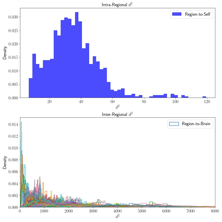
Empirical distributions of within-region (top) and between-region (bottom) $$d^{2}$$ values. Each line is the distribution of the distance of samples in our ROI to a whole region.

As expected, the distribution of $d^{2}$ the distance of samples in our region of interest, $l_{T}$ , to distributions computed from other regions are (considerably) larger and much more variable, while the profile of points within $l_{T}$ looks to have much smaller variance – this is good! This means that we have high intra-regional similarity when compared to inter-regional similarities. This fits what’s known in neuroscience as the “cortical field hypothesis”.

Step 2: Distributional QC-Check

Because we know that our data should follow a $\chi^{2}_{p}$ distribution, we can fit the MLE estimate of our location and scale parameters, while keeping the $df$ parameter fixed.

p = data_lt.shape[1]
mle_chi2_theory = chi2.fit(dist_lt2, fdf=p)

xr = np.linspace(data_lt.min(), data_lt.max(), 1000)
pdf_chi2_theory(xr, *mle_chi2_theory)

fig = plt.subplot(1,2,2,figsize=(18, 6))

# plot theoretical vs empirical null distributon
plt.subplot(1,2,1)
plt.hist(data_lt, density=True, color='blue', alpha=0.6,
    label = 'Empirical')
plt.plot(xr, pdf_chi2_theory, color='red',
    label = '$\chi^{2}_{p}')

# plot QQ plot of empirical distribution
plt.subplot(1,2,2)
probplot(D2.squeeze(), sparams=mle_chi2_theory, dist=chi2, plot=plt);

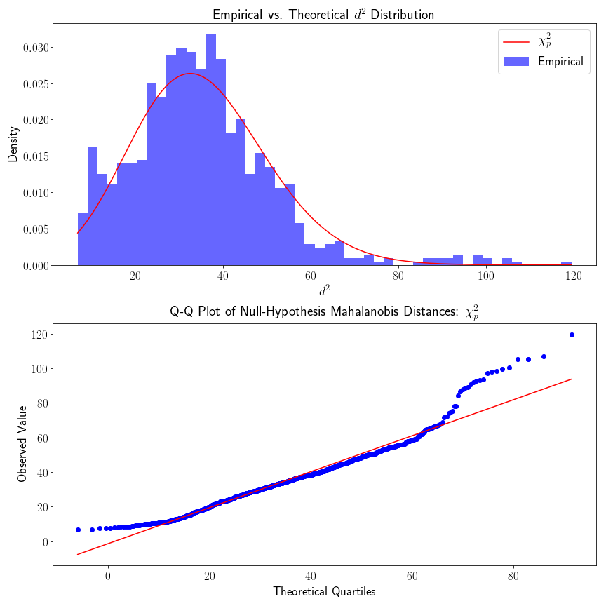
Density and QQ plot of null distribution.

From looking at the QQ plot, we see that the empirical density fits the theoretical density pretty well, but there is some evidence that the empirical density has heavier tails. The heavier tail of the upper quantile could probability be explained by acknowledging that our starting cortical map is not perfect (in fact there is no “gold-standard” cortical map). Cortical regions do not have discrete cutoffs, although there are reasonably steep gradients in connectivity. If we were to include samples that were considerably far away from the the rest of the samples, this would result in inflated densities of higher $d^{2}$ values.

Likewise, we also made the distributional assumption that our connectivity vectors were multivariate normal – this might not be true – in which case our assumption that $d^{2}$ follows a $\chi^{2}_{p}$ would also not hold.

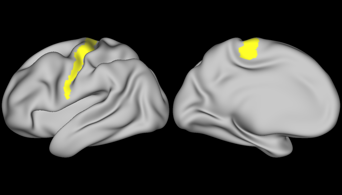
Finally, let’s have a look at some brains! Below, is the region we used as our target – the connectivity profiles from vertices in this region were used to compute our mean vector and covariance matrix – we compared the rest of the brain to this region.

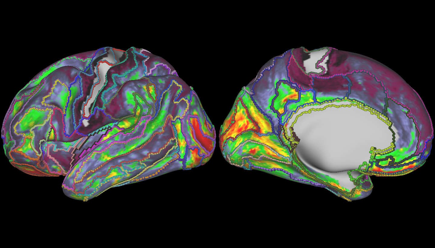
Estimated squared Mahalanobis distances, overlaid on cortical surface.

Here, larger $d^{2}$ values are in red, and smaller $d^{2}$ are in black. Interestingly, we do see pretty large variance of $d^{2}$ spread across the cortex – however the values are smoothly varying, but there do exists sharp boundaries. We kind of expected this – some regions, though geodesically far away, should have similar connectivity profiles if they’re connected to the same regions of the cortex. However, the regions with connectivity profiles most different than our target region are not only contiguous (they’re not noisy), but follow known anatomical boundaries, as shown by the overlaid boundary map.

This is interesting stuff – I’d originally intended on just learning more about the Mahalanobis Distance as a measure, and exploring its distributional properties – but now that I see these results, I think it’s definitely worth exploring further!

← Previous Post Next Post →