The Delta Method - A Rambling On

Here, we’ll look at various applications of the Delta Method, especially in the context of variance stabilizing transformations, along with looking at the confidence intervals of estimates.

The Delta Method is used as a way to approximate the Standard Error of transformations of random variables, and is based on a Taylor Series approximation.

In the univariate case, if we have a random variable, $X_{n}$ , that converges in distribution to a $N(0, \sigma^{2})$ distribution, we can apply a function to this random variable as:

$\begin{align} \sqrt{n}(X_{n} - \theta) \xrightarrow{d} N(0,\sigma^{2}) \\ \sqrt{n}(g(X_{n}) - g(\theta)) \xrightarrow{d} \; ? \end{align}$

However, we don’t know the asymptotic variance of this transformed variable just yet. In this case, we can approximate our function $g(x)$ using a Taylor Series approximation, evaluated at $\theta$ :

$\begin{align} g(x) = g(\theta) + g\prime(\theta)(x-\theta) + O() \end{align}$

where $O()$ is the remainder of higher-order Taylor Series terms that converges to 0.

By Slutsky’s Theorem and the Continious Mapping Theorem, we know that since $\bar{\theta} \xrightarrow{p} \theta$ , we know that $g\prime(\bar{\theta}) \xrightarrow{p} g\prime(\theta)$

Plugging this back in to our original equation and applying Slutsky’s Perturbation Theorem, we have:

$\begin{align} &= \sqrt{n}(\Big[g(\theta) + g\prime(\theta)(x-\theta)\Big] - g(\theta)) \\ &= \sqrt{n}(g\prime(\theta)(x-\theta)) \\ &= g\prime(\theta)\sqrt{n}(X_{n} - \theta) \end{align}$

and since we know that $\sqrt{n}(\bar{X_{n}} - \theta) \xrightarrow{d} N(0,\sigma^{2})$ , we now know that $g\prime(\theta) \sqrt{n}(\bar{X_{n}} - \theta) \xrightarrow{d} N(0,g\prime(\theta)^{2} \sigma^{2})$ . As such, we have that:

$\begin{align} \sqrt{n}(g(X_{n}) - g(\theta)) \xrightarrow{d} N(0, g\prime(\theta)^{2}\sigma^{2}) \end{align}$

The Delta Method can be generalized to the multivariate case, where, instead of the derivative, we use the gradient vector of our function:

$\begin{align} \sqrt{n}(g(\bar{X_{n}} - g(\theta)) \xrightarrow{d} N(0, \nabla(g)^{T} \Sigma \nabla(g)) \end{align}$

Below, I’m going to look at a few examples applying the Delta Method to simple functions of random variables. Then I’ll go into more involved examples applying the Delta Method via Variance Stabilizing Transformations. Oftentimes, the variance of an estimate depends on its mean, which can vary with the sample size. In this case, we’d like to find a function $g(\theta)$ , such that, when applied via the Delta Method, the variance is constant as a function of the sample size.

We’ll start by importing the necessary libraries and defining two functions:

%matplotlib inline
import matplotlib.pyplot as plt

from matplotlib import rc
rc('text', usetex=True)

from scipy.stats import norm, poisson, expon
import numpy as np

Here, we define two simple functions – one to compute the difference between our estimate and its population paramter, and the other to compute the function of our random variable as described by the Central Limit Theorem.

def conv_prob(n, est, pop):
    
    """
    Method to compute the estimate for convergence in probability.
    """
    
    return (est-pop)

def clt(n, est, pop):
    
    """
    Method to examine the Central Limit Theorem.
    """
    
    return np.sqrt(n)*(est-pop)

Let’s have a look at an easy example with the Normal Distribution. We’ll set $\mu = 0$ and $\sigma^{2} = 5$ . Remember that when using the Scipy Normal distribution, the norm class accepts the standard deviation, not the variance. We’ll show via the Central Limit Theorem that the function $\sqrt{n}(\bar{X_{n}} - \mu) \xrightarrow{d} N(0,\sigma^{2})$ .

# set sample sample sizes, and number of sampling iterations
N = [5,10,50,100,500,1000]
iters = 500

mu = 0; sigma = np.sqrt(5)

# store estimates
norm_clt = {n: [] for n in N}

samples = norm(mu,sigma).rvs(size=(iters,1000))

for n in N:
    for i in np.arange(iters):
        
        est_norm = np.mean(samples[i,0:n])
        norm_clt[n].append(clt(n, est_norm, mu))

Now let’s plot the results.

# Plot results using violin plots
fig = plt.subplots(figsize=(8,5))

for i,n in enumerate(N):
    temp = norm_clt[n]
    m = np.mean(temp)
    v = np.var(temp)
    print('Sample Size: %i has empirical variance: %.2f' % (n, v.mean()))
        
    plt.violinplot(norm_clt[n], positions=[i],)

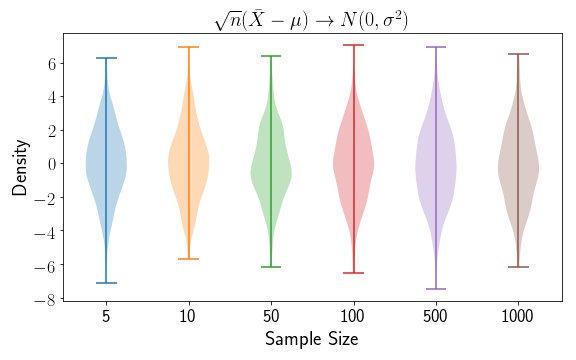
Central Limit Theorem applied to Normal Distribution.

As expected, we see that the Normal distribution mean and variance estimates are independent of the sample size. In this case, we don’t need to apply a variance stabiliing transformation. We also see that the variance fluctuates around $5$ . Now, let’s apply a simple function $g(\theta) = \theta^{2}$ to our data. So $g\prime(\theta) = 2\theta$ , and the variance of our function becomes $g\prime(\mu)^{2}\sigma^{2} = (2\mu)^{2} \sigma^{2} = 4\mu^{2}\sigma^{2}$ . Let’s look at a few plots, as a function of changing $\mu$ .

# set sample sample sizes, and number of sampling iterations
mus = [1,2,3,4]

N = [5,10,50,100,500,1000]
iters = 2000
sigma = np.sqrt(5)


fig, ([ax1,ax2], [ax3,ax4]) = plt.subplots(2,2, figsize=(14,9))
for j ,m in enumerate(mus):
    
    # store estimates
    norm_clt = {n: [] for n in N}
    samples = norm(m, sigma).rvs(size=(iters, 1000))
    
    
    plt.subplot(2,2,j+1)
    for k, n in enumerate(N):
        np.random.shuffle(samples)
        for i in np.arange(iters):

            est_norm = np.mean(samples[i, 0:n])
            norm_clt[n].append(clt(n, est_norm**2, m**2))

        plt.violinplot(norm_clt[n], positions=[k],)

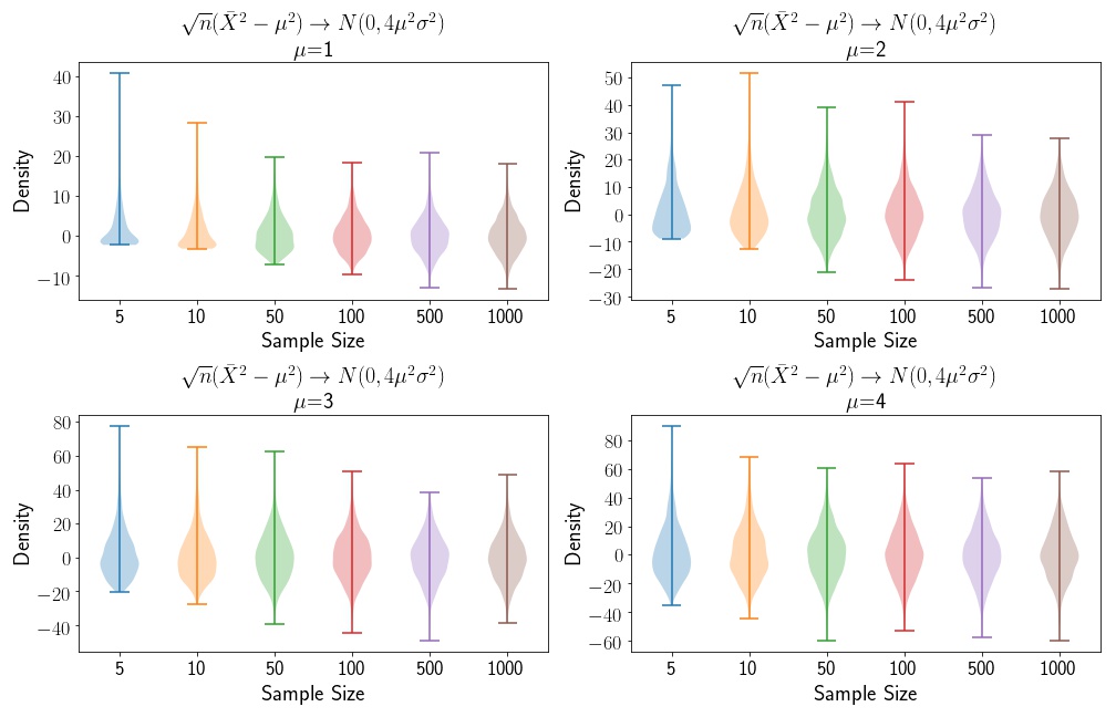
Central Limit Theorem applied to function of Normal Distribution.

We see that the variance increases as the mean increases, and that, as the sample sizes increase, the distributions converge to the $N(0, 4\mu^{2}\sigma^{2})$ asymptotic distribution.

Variance Stabilization for the Poisson Distribution

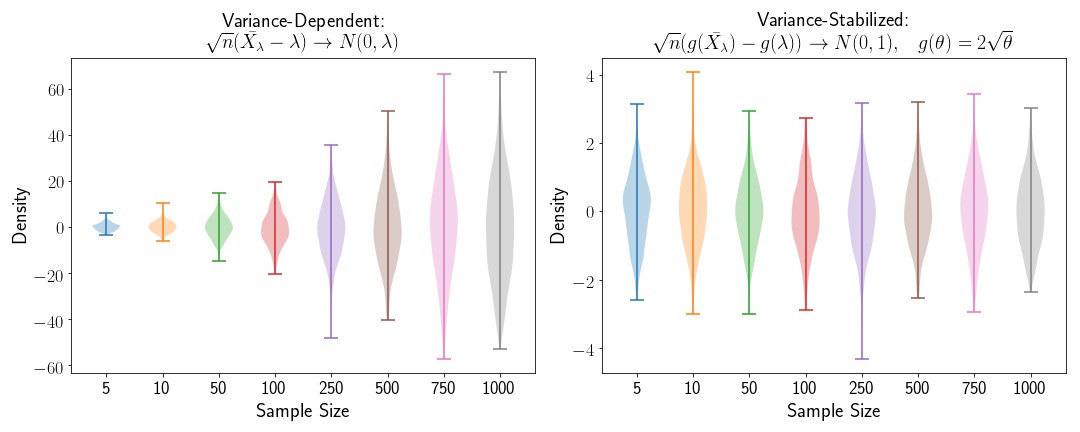
Now let’s look at an example where the variance depends on the sample size. We’ll use the Poisson distribution in this case. We know that for the Poisson distribution, the variance is dependent on the mean, so let’s define a random variable, $X_{\lambda}$ , where $\lambda = n*\theta$ . $n$ is the sample size, and $\theta$ is a fixed constant.

We’ll define $X_{\lambda } = \sum_{i=1}^{n} X_{\theta}$ , the sum of $n$ independent Poisson random variables, so that the expected value and variance of $X_{\lambda } = n\theta$

If we wanted to apply the Central Limit Theorem to $X_{\lambda }$ , our convergence would be as follows:

$\begin{align} \sqrt{n}(X_{\lambda} - \lambda) \xrightarrow{d} N(0,\sigma^{2}(\lambda)) \end{align}$

where the variance $\sigma^{2}(\lambda)$ depends on the mean, $\lambda$ . In order to stabilize the variance of this variable, we can apply the Delta Method, in order to generate a variable that converges to a standard Normal distribution asymptotically.

$\begin{align} \sqrt{n}(g(X_{\lambda}) - g(\lambda)) \xrightarrow{d} N(0,g\prime(\theta)^{2}\sigma^{2}) \\ \end{align}$

where

$\begin{align} &g\prime(\theta)^{2} \theta = 1 \\ &g\prime(\theta)^{2} = \frac{1}{\theta} \\ &g\prime(\theta) = \frac{1}{\sqrt{\theta}} \\ &g(\theta) = \int \frac{\partial{\theta}}{\sqrt{\theta}} \\ &g(\theta) = 2\sqrt{\theta} \end{align}$

is our variance stabilizing function.

def p_lambda(n, theta=0.5):
    
    """
    Function to compute lambda parameter for Poisson distribution.
    Theta is constant.
    """
    return n*theta

theta = 0.5

N = [5,10,50,100,250,500,750,1000]
iters = 500

clt_pois = {n: [] for n in N}
pois_novar= {n: [] for n in N}
pois_var = {n: [] for n in N}

for n in N:
    for i in np.arange(iters):
        est_mu = np.mean(poisson(mu=(n*theta)).rvs(n))

        pois_novar[n].append(clt(n, est_mu, p_lambda(n)))
        pois_var[n].append(clt(n, 2*np.sqrt(est_mu), 2*np.sqrt(p_lambda(n))))
        
        clt_pois[n].append(conv_prob(n, est_mu, n*theta))

fig,([ax1, ax2]) = plt.subplots(2,1, figsize=(15,6))

plt.subplot(1,2,1)
for i,n in enumerate(N):
    plt.violinplot(pois_novar[n], positions=[i])

plt.subplot(1,2,2)
for i,n in enumerate(N):
    plt.violinplot(pois_var[n], positions=[i])

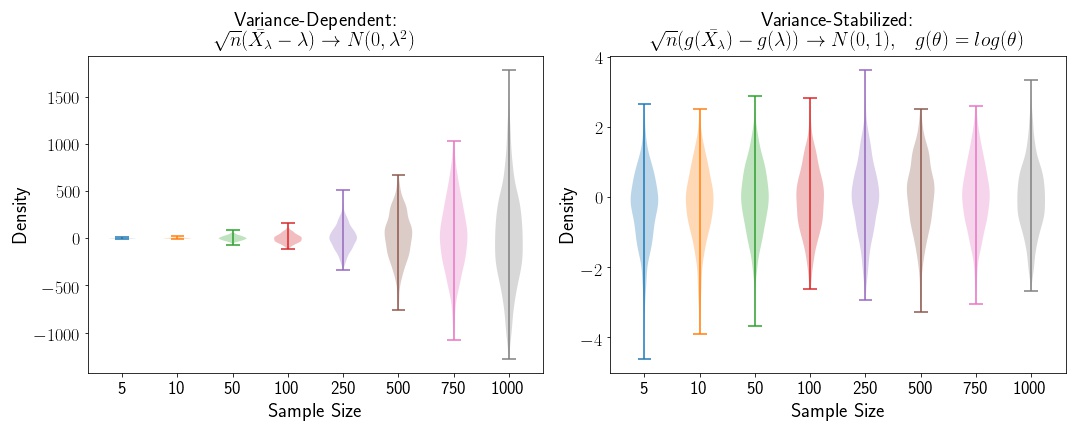
Variance stabilization of Poisson distribution.

Variance Stabilization for the Exponential Distribution

Applying the same method to the Exponential distribtuion, we’ll find that the variance stabilizing transformation is $g(\theta) = log(\theta)$ . We’ll apply that here:

theta = 0.5

N = [5,10,50,100,250,500,750,1000]
iters = 500

clt_exp = {n: [] for n in N}
exp_novar= {n: [] for n in N}
exp_var = {n: [] for n in N}

for n in N:
    for i in np.arange(iters):
        samps = expon(scale=n*theta).rvs(n)
        
        est_mu = np.mean(samps)
        est_var = np.var(samps)

        exp_novar[n].append(clt(n, est_mu, (n*theta)))
        exp_var[n].append(clt(n, np.log(est_mu), np.log(n*theta)))
        
        clt_exp[n].append(conv_prob(n, est_mu, n*theta))

fig,([ax1, ax2]) = plt.subplots(2,1, figsize=(15,6))

plt.subplot(1,2,1)
for i,n in enumerate(N):
    plt.violinplot(exp_novar[n], positions=[i])

plt.subplot(1,2,2)
for i,n in enumerate(N):
    plt.violinplot(exp_var[n], positions=[i])

Variance stabilization of Exponential distribution.

Example of Standard Error Computation Using Delta Method for Polynomial Regression

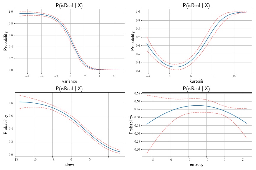
As an example of applying the Delta Method to a real-world dataset, I’ve downloaded the banknote dataset from the UCI Machine Learning Repository. In this exercise, I’ll apply the logistic function via logistic regression to assess whether or not a banknote is real or fake, using a set of features. I’ll compute confidence intervals of our prediction probabilities using the Delta Method. There are four unique predictors in this case: the variance, skew, kurtosis, and entropy of the Wavelet-transformed banknote image. I’ll treat each of these predictors independently, using polynomial basis function of degree $3$ .

In this example, we’re interested in the standard error of our probability estimate. Our function is the Logistic Function, as follows:

$\begin{align} g(\beta) &= \frac{1}{1+e^{-x^{T}\beta}} \\ &= \frac{e^{x^{T}\beta}}{1+e^{x^{T}\beta}} \end{align}$

where the gradient of this multivariate function is:

$\begin{align} \nabla g(\beta) &= \frac{\partial g}{\partial \beta} e^{x^{T}\beta}(1+e^{x^{T}\beta})^{-1} \\ &= x^{T}e^{x^{T}\beta}(1+e^{x^{T}\beta})^{-1} - x^{T}e^{x^{T}\beta}e^{x^{T}\beta} \\ &= x^{T}\Big(e^{x^{T}\beta}(1+e^{x^{T}\beta})^{-1} - e^{x^{T}\beta}e^{x^{T}\beta}\Big)(1+e^{x^{T}\beta})^{-2} \\ &= x^{T} \frac{e^{x^{T}\beta}}{(1+e^{x^{T}\beta})^{2}} \\ \nabla g(\beta) &= x^{T} g(\beta)(1-g(\beta)) \end{align}$

so that the final estimate of our confidence interval becomes

$\begin{align} & \sim N(0,x^{T} g(\beta)(1-g(\beta)) \Sigma g(\beta)(1-g(\beta))x) \\ & \sim N(0, \nabla g(\beta)^{T} \Sigma \nabla g(\beta)) \end{align}$

import pandas as pd
import statsmodels.api as sm
from sklearn.preprocessing import PolynomialFeatures

import pandas as pd
import statsmodels.api as sm
from sklearn.preprocessing import PolynomialFeatures

bank = pd.read_csv('/Users/kristianeschenburg/Documents/Statistics/BankNote.txt',
                   sep=',',header=None, names=['variance', 'skew', 'kurtosis', 'entropy','class'])
bank.head()

fig = plt.subplots(2,2, figsize=(12,8))
for j, measure in enumerate(['variance', 'kurtosis', 'skew', 'entropy']):

    predictor = np.asarray(bank[measure])
    response = np.asarray(bank['class'])
    
    idx = (response == 1)

    # plot test set
    plt.subplot(2,2,j+1)
    plt.violinplot(predictor[idx], positions=[1]);
    plt.violinplot(predictor[~idx], positions=[0])
    plt.title('{:} By Classification'.format(measure), fontsize=18)
    plt.ylabel('Measure: {:}'.format(measure),fontsize=15)
    plt.yticks(fontsize=13)
    plt.xticks([0,1],['Fake','Real'], fontsize=15)

plt.tight_layout()

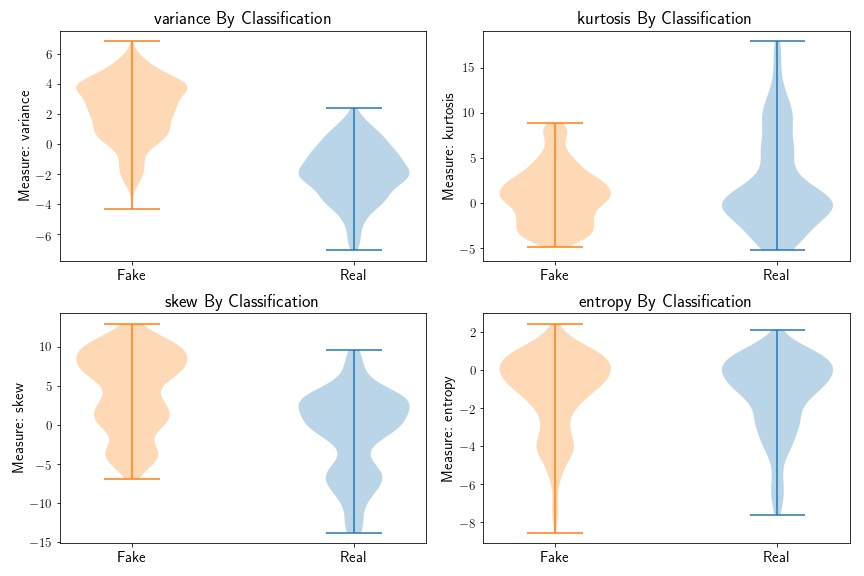
Bank note feature distributions, based on note class.

Based on the above plot, we can see that variance, skew, and kurtosis seem to be the most informative, while the entropy distributions do not seem to be that different based on bank note class.

Next, we fit a logistic regression model of note classification on note feature, with polynomial order of degree 3. We then compute the standard errors of the transformed variance. It was transformed using the logistic function, so we’ll need to compute the gradient of this function.

fig = plt.subplots(2,2, figsize=(12,8))
for j, measure in enumerate(['variance', 'kurtosis', 'skew', 'entropy']):

    # Generate polynomial object to degree 
    # transform age to 4-degree basis function
    poly = PolynomialFeatures(degree=2)
    idx_order = np.argsort(bank[measure])

    predictor = bank[measure][idx_order]
    response = bank['class'][idx_order]

    features = poly.fit_transform(predictor.values.reshape(-1,1));

    # fit logit curve to curve
    logit = sm.Logit(response, features).fit();
    
    test_features = np.linspace(np.min(predictor), np.max(predictor), 100)
    test_features = poly.fit_transform(test_features.reshape(-1,1))
    # predict on test set
    class_prob = logit.predict(test_features)

    cov = logit.cov_params()
    yx = (class_prob*(1-class_prob))[:,None] * test_features
    se = np.sqrt(np.diag(np.dot(np.dot(yx, cov), yx.T)))

    # probability can't exceed 1, or be less than 0
    upper = np.maximum(0, np.minimum(1, class_prob+1.96*se))
    lower = np.maximum(0, np.minimum(1, class_prob-1.96*se))

    # plot test set
    plt.subplot(2,2,j+1)
    plt.plot(test_features[:, 1], class_prob);
    plt.plot(test_features[:, 1], upper, color='red', linestyle='--', alpha=0.5);
    plt.plot(test_features[:, 1], lower, color='red', linestyle='--', alpha=0.5);
    plt.title(r'P(isReal \Big| X)', fontsize=18)
    plt.xlabel('{:}'.format(measure),fontsize=15)
    plt.ylabel('Probability',fontsize=15)
    plt.grid(True)

plt.tight_layout()

Confidence intervals for each feature, computed using Delta Method.

← Previous Post Next Post →